---
bibliography:
- lib/zotero.bib
link-citations: true
mainfont: Linux Libertine O
monofont: DejaVu Sans Mono
sansfont: Linux Biolinum O
title: Clear Skies - A Reference Architecture for Resilient Alaskan
Microgrid Cyberinfrastructure
title-block: false
---
Basic Book Builder
A Pandoc Template for building books and articles
| Title | Basic Book Builder |
| Subtitle | A Pandoc Template for building books and articles |
| Affiliation | Alaska Center for Energy and Power |
| Institution | University of Alaska Fairbanks |
| Author | John Haverlack |
| Copyright | © 2025 Alaska Center for Energy and Power |
| License | CC BY-ND 4.0 |
| Version | 1.0.0 |
| Date | 2025-11-13 |
| State | BETA |
| Source | https://github.com/jehaverlack/basic-book-builder |
- [Introduction](#introduction)
- [Conventions](#conventions)
- [Getting Started](#getting-started)
- [Installing Pre-Requisites](#installing-pre-requisites)
- [Required](#required)
- [Optional](#optional)
- [Editing the Configuration](#editing-the-configuration)
- [Editing the Book](#editing-the-book)
- [Configuration](#configuration)
- [FrontMatter Config](#frontmatter-config)
- [Editing the Content](#editing-the-content)
- [Citations](#citations)
- [Usage: Building the Book](#usage-building-the-book)
- [Example Content](#example-content)
- [SI Conversion Factors](#si-conversion-factors)
- [Physical Constants](#physical-constants)
- [Fine Structure Constant](#fine-structure-constant)
- [Newton’s Law of Gravity](#newtons-law-of-gravity)
- [Relativistic Energy Momentum
Relation](#relativistic-energy-momentum-relation)
- [Planck’s Constant](#plancks-constant)
- [Planck Length](#planck-length)
- [Fine Structure Constant](#fine-structure-constant-1)
- [Sage Code](#sage-code)
- [Terminology](#terminology)
- [Citations](#citations-1)
# Introduction
This is a basic book (or article) builder template based on a Pandoc
build process in conjunction with a number of other tools to generate
PDF, ODT, HTML, LaTex, Markdown, and Epub book output formats from
Markdown source content , which can optionally be edited as an Obsidian
vault.
This book builder template has been curated by John Haverlack.([“John
Haverlack ACEP” n.d.](#ref-JohnHaverlackACEP))
## Conventions
A few callout box styles have been added to easily highlight content.
**Established Concept**
Einsteins Relativistic Dynamics Equations
*E*2 = (*m*0⋅*c*2)2 + (*p*⋅*c*)2
**Proposed Concept**
With the speed of light, *c* = 1:
*E*2 = *m*02 + *p*2
**Speculative Concept**
With the speed of light, *c* = 1:
*E*2 = *m*02 + *p*2
**Caution Note**
Beware of this section.
**Warning Note**
Beware of this section.
**Alerts**
Extreme Highlight
# Getting Started
## Installing Pre-Requisites
For Debian / ZorinOS and likely Ubuntu based systems.
**TODO**
It would be nice to roll a setup script to take care of this.
### Required
#### Pandoc
- https://pandoc.org/
- [Download](https://github.com/jgm/pandoc/releases/tag/3.8.2.1)
sudo apt install https://github.com/jgm/pandoc/releases/download/3.8.2.1/pandoc-3.8.2.1-1-amd64.deb
#### Code Editor
**Code Editor**
[VSCodium](https://vscodium.com/) is recommend for privacy
(telemetry/tracking) reasons - https://vscodium.com/
But any text editor will work. \#### make
sudo apt install make
#### jq and yq
sudo apt install jq yq
#### texlive
sudo apt install texlive texlive-xetex texlive-latex-extra texlive-fonts-recommended texlive-fonts-extra
#### MathJax
- https://www.mathjax.org/
wget https://registry.npmjs.org/mathjax/-/mathjax-3.2.2.tgz
tar xzf mathjax-3.2.2.tgz
mv package/es5/* lib/mathjax
rm -rf package mathjax-3.2.2.tgz
**TODO**
This need to be rolled into a setup script.
### Optional
The following are not strictly requires to use this book builder
template.
#### Obsidian
**Highly Recommended**
Editing book chapter content in Obsidian is a very productive means for
editing Markdown source content.
- https://obsidian.md/
- [Deb
Package](https://github.com/obsidianmd/obsidian-releases/releases/download/v1.9.14/obsidian_1.9.14_amd64.deb)
sudo apt install https://github.com/obsidianmd/obsidian-releases/releases/download/v1.9.14/obsidian_1.9.14_amd64.deb
#### Zotero
**Highly Recommended**
If you need to managed citations and references, Zotero integration is
highly recommended.
- https://www.zotero.org/
sudo cp ./scripts/deps/zotero.list /etc/apt/sources.list.d/
sudo apt update
sudo apt install zotero
##### Better BibTex for Zotero
Install the Better BibTex Plugin for Zotero - Zotero \> Tool \> Plugins
##### Export citations.bib
- Zotero \> File \> Export Library \> Format: Better BibTeX
- [ ] Keep Updated
- [ ] Save to: \~/Documents/Lib/zotero.bib
- [ ] Symlink your \~/Documents/Lib/Citations.bib to
basic-book-builder/lib/zotero.bib
##### Zotero Connector Browser Plugin
- https://chromewebstore.google.com/detail/zotero-connector/ekhagklcjbdpajgpjgmbionohlpdbjgc
Provides you the ability to auto add Web resources to your Zotero
citation database.
#### lmodern
sudo apt install lmodern
#### epubcheck
sudo apt install epubcheck
#### foliate
An EPub Reader
- https://johnfactotum.github.io/foliate/
sudo apt install https://github.com/johnfactotum/foliate/releases/download/2.6.4/com.github.johnfactotum.foliate_2.6.4_all.deb
#### calibre
An EPub Reader
- https://calibre-ebook.com
sudo apt install calibre
## Editing the Configuration
# Editing the Book
### Configuration
There are a number of other config files for each format:
conf/
├── epub-metadata.xml
├── epub_template.html
├── epub.yaml
├── frontmatter_epub.md
├── frontmatter_epub.xhtml
├── frontmatter.html
├── frontmatter.tex
├── header.tex
├── html.yaml
├── latex.yaml
├── markdown.yaml
├── metadata.yaml
├── pandoc.yaml
├── pdf.yaml
├── style.css
└── style_epub.css
#### Main Config Files
- metadata.yaml - Set Title, etc
- pandoc.yaml - Main Pandoc Config \#### Per format Configs
- `pdf.yaml`
- `html.yaml`
- `latex.yaml`
- `epub.yaml`
### FrontMatter Config
There are 2 Version of the FrontMatter for PDF, and HTML bases formats
that set the Title, Author, Verizon, Copyright, etc…
- `frontmatter.tex`
- `frontmatter.html`
- `frontmatter_epub.*` - Work in Progress
> There is probably a better way to do this.
## Editing the Content
To edit the book open the `basic-book-builder` directory as an Obsidian
Vault.
- Edit the Markdown content in the `chapters` directory.
### Citations
> Note: the Zotero database needs configured to export automatically to
> `lib/citations.bib`
To insert a Zotero Citation - Ensure the Zotero App and DB are running
on you system. - Alt + I (to insert citation) - Search for and select
citation reference
## Usage: Building the Book
#### PDF
make pdf
#### HTML
make html
#### LaTex
make latex
#### Markdown
make markdown
#### EPub
> Note: This ePub configuration still needs tuning.
make epub
# Example Content
In *R**ν* the [Planck
Length](https://en.wikipedia.org/wiki/Planck_units#Planck_length) is the
universal unit for measurement of distance, and is defined approximately
to be:
$$\\boxed{L_P=\\sqrt{\\hbar}=5.72928\\times10^{-35}m=1 L}$$
Where 1 *L*, is 1 Planck Length of distance.
### SI Conversion Factors
The following conversion factors can be used to convert observable
quantities of measure from the *SI* system of units to *R**ν* to \~6
significant digits.
| Conversion Factor | Symbol | Value |
|------------------------------|-------------------|--------------------------------------------------------|
| meters to Planck Length | *χ**P* | $1.74542\\times10^{34} \\frac{L}{m}$ |
| seconds to Planck Length | *τ**p* | $5.23264\\times10^{42} \\frac{L}{s}$ |
| mass to Planck Length | *G**P* | $1.62871\\times10^8 \\frac{L}{kg}$ |
| energy to Planck Length | *E**P* | $1.81219\\times10^9 \\frac{L}{J}$ |
| momentum to Planck Length | *P**P* | $5.43280\\times10^{-1} \\frac{L\\cdot s}{kg \\cdot m}$ |
| temperature to Planck Length | *k**P* | $2.501998\\times10^{-14} \\frac{L}{K}$ |
| charge to Planck Length | *C**P* | $1.89007\\times10^{18} \\frac{L}{C}$ |
### Physical Constants
Applying conversion factors from the table above, we can convert SI
values to Reduced Natural Units. For example, performing this analysis
on the the speed of light yields a unit-less number with a value of 1:
$c = 299792458 \\frac{m}{s} = 299792458 \\frac{m}{s} \\cdot 1.74542\\times10^{34} \\frac{L}{m} \\cdot \\frac{1}{5.23264\\times10^{42} \\frac{L}{s}} = 1.00000$
| Quantity | Symbol | SI | *ν* |
|--------------------------------|-------------------|-----------------------------------------------------------------|-----------------------------------------|
| Speed of Light | *c* | $299792458 \\frac{m}{s}$ | 1 |
| Reduced Gravitational Constant | *G*0 | $8.38659\\times10^{-10} \\frac{m^3}{kg \\cdot s^2}$ | 1 |
| Boltzmann’s Constant | *k* | $k=1.380649\\times10^-23 \\frac{J}{K}$ | 1 |
| Permittivity of Free Space | *ϵ**o* | $8.854187817620\\times10^{-12} \\frac{C^{2}s^2}{kg \\cdot m^3}$ | 1 |
| Permeability of Free Space | *μ**o* | $\\huge{\\frac{1}{\\epsilon\_{o} \\cdot c^{2}}}$ | 1 |
| Reduced Planck’s Constant | ℏ | $1.054571726\\times10^-34 \\frac{kg \\cdot m^2}{s}$ | 1*L*2 |
| Mass of the Electron | *m**e* | 9.10938 × 10⁻³¹*k**g* | 1.48366 × 10⁻²²*L* |
| Charge of the Electron | *e*− | − 1.60218 × 10⁻¹⁹*C* | − 3.02822 × 10⁻¹*L* |
| Unit Cycle | *Θ* | 2*π* = 6.28318... *R**a**d**i**a**n**s* | 1*τ* = 6.28318... *R**a**d**i**a**n**s* |
## Fine Structure Constant
As a consistency check, we compute the *[Fine Structure
Constant](https://en.wikipedia.org/wiki/Fine-structure_constant)* using
Reduced Natural Units which is a unit less ratio that should be
independent of our system of units.
$\\huge{\\alpha=\\frac{e^2}{4\\pi\\epsilon_o\\hbar c}=\\frac{e^2}{2\\tau}=0.00729735≈\\frac{1}{137}}$
#### Dimensional Analysis
The reader should be familiar with high school physics and chemistry
[dimensional
analysis](https://en.wikipedia.org/wiki/Dimensional_analysis).
- 1 *m**e**t**e**r* (*m*) = 100 *c**e**n**t**i**m**e**t**e**r**s* (*c**m*)
- 1 *k**i**l**o**m**e**t**e**r* (*k**m*) = 1000 *m**e**t**e**r**s* (*m*)
- 1 *m**i**l**e* = 5280 *f**e**e**t* (*f**t* *o**r* ′)
- $1\\ foot\\ (ft\\ or\\ ') = 12\\ inches\\ (in\\ or\\ ")$
- $1\\ inch\\ (") = 2.54\\ centimeters\\ (cm)$
How many kilometers are in 1 mile?
$1\\ mile = 1\\ mile \\times \\frac{5280\\ ft}{mile} \\times \\frac{12\\ in}{ft} \\times \\frac{2.54\\ cm}{in}\\times \\frac{1\\ m}{100 cm} \\times \\frac{1\\ km}{1000 m} = \\frac{5280 \\times 12 \\times 2.54}{100 \\times 1000}\\ km = \\frac{160934.40}{100000}\\ km = 1.6\\ km$
Note that each unit in the denominator cancels with one if the numerator
until we are left with only km.
## Newton’s Law of Gravity
The force of gravity (*F**g*) between 2 masses, *m*1 and *m*2
separated by distance *r* is given by [Newton’s Law of
Gravity](https://en.wikipedia.org/wiki/Newton%27s_law_of_universal_gravitation):
$F\_{g} = G \\frac{m\_{1} m\_{2}}{r^{2}}$
Where *G*, is the [Gravitational
Constant](http://en.wikipedia.org/wiki/Gravitational_Constant).
$G = 6.67430 \\times 10^{-11}\\ N\\frac{m^2}{kg^2}$
The strength of gravitational force follow the inverse square law
distributing gravitational flux over the surface area of a sphere
(4*π**r*2).
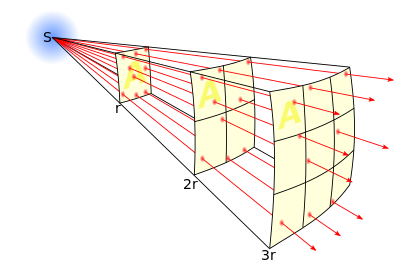
#### Inverse Square Law
Any source of a signal strength (*S*0) that radiates
isotropically in 3-dimensional space will distribute that signal
strength (*S*0) over the surface area of a sphere
(*S**A* = 4*π**r*) of radius (*r*). Such that the intensity (*I*) at
distance (*r*) is:
$$I(r) = \\frac{S_0}{4 \\pi r^{2}}=\\frac{S_0}{2 \\tau r^{2}}$$
 \#### *R**ν*
Reduced Gravitational Constant In this version of Newton’s Law of
Gravity we introduce a new constant *G*0, the reduced
gravitational constant to accommodate for the factor of 4*π* = 2*τ*
which is has been integrated in the SI version of the gravitational
constant.
$F_g =G \\frac{m\_{1} m\_{2}}{r^{2}}= G_0 \\frac{m\_{1} m\_{2}}{4 \\pi r^{2}}=G_0 \\frac{m\_{1} m\_{2}}{2 \\tau r^{2}}$
Where:
$G = \\frac{G\_{0}}{2\\tau} = 6.67384 \\times 10^{-11} \\frac{N \\cdot m^2}{kg^2}$
Analyzing the units:
$$\\frac{N \\cdot m^2}{kg^2} = \\left( \\frac{\\left( kg \\cdot \\frac{m}{s^2} \\right) \\cdot m^2}{kg^2} \\right)=\\frac{m^3}{s^2 kg}$$
Converting seconds to meters with the SI speed of light as a conversion
factor:
$$\\frac{m^3}{s^2 kg}\\cdot\\frac{1}{c^2}=\\frac{m^3}{s^2 kg}\\cdot\\frac{s^2}{m^2}=\\frac{m}{kg}$$
Thus where space and time are measured in units of meters, the reduced
gravitational constant, is:
$$\\boxed{G_0=\\frac{2\\tau G}{c^2}=\\frac{2\\tau \\cdot 6.67384 \\times 10^{-11}}{299792458^2} \\frac{m}{kg} = 9.33135 \\times 10^-27 \\frac{m}{kg}}$$
> Observation This implies that not only can space an time be measure in
> units of meters, but so can mass.
### Relativistic Energy Momentum Relation
Einsteins [Relativistic Energy
Momentum](https://en.wikipedia.org/wiki/Energy%E2%80%93momentum_relation)
relationship shows a Pythagorean relation between the total energy
(*E*), rest mass (*m*0) and momentum (*p*) of a system.
*E*2 = (*m*0⋅*c*2)2 + (*p*⋅*c*)2
Where space and time are both measure in units of meters, c=1.
*E*2 = (*m*0)2 + (*p*)2
From this we can see that Energy, Momentum and Mass have equivalent
units.
> *While we do not really know what energy, mass and momentum are we
> know that they are fundamentally “made” out of the same stuff because
> they have the same units.*
##### Objects of mass at rest
For an object at rest with no momentum (*p* = 0) we see Einstein’s
famous equations:
*E* = *m*0 ⋅ *c*2
Or, with *c* = 1, this is much simpler to understand. Energy = Mass
*E* = *m*0
##### Zero mass objects moving at the speed of light
And for objects with no mass, like photos, (*m*0 = 0):
*E* = *p**c*
Or, with *c* = 1, this is much simpler to understand. Energy = Momentum
*E* = *p*
## Planck’s Constant
The [Reduced Planck
constant](https://en.wikipedia.org/wiki/Planck_constant) , ħ, represents
a conversion factor for relating the frequency, *ω* (in 2*π* radians per
second), of a photon to the energy of that photon. This can easily be
seen from the simple but profound relationship:
*E* = ℏ*ω*
Where:
ℏ = 1.054571726 × 10⁻³⁴*J* ⋅ *s*
and
$J \\cdot s = {kg}\\cdot\\frac{m^2}{s}$
> Reduced Planck’s Constant
> $\\hbar = \\frac{h}{2\\pi} = \\frac{h}{\\tau}$
Simplifying our units by converting time and mass to units of meters:
$$\\boxed{\\hbar=1.054571726 \\times 10^{−34} {kg}\\cdot\\frac{m^2}{s}\\cdot\\frac{G_0}{c}=3.282462\\times10^{-69}m^2}$$
Which suggest that the Plank constant can be interpreted as an areas for
which the square root of is suspiciously close to the Plank length:
$$\\boxed{\\sqrt{\\hbar}=\\sqrt{3.282462\\times10^{-69}m^2}=5.72928\\times10^{-35}m}$$
#### Planck Area
The [Planck
Area](https://en.wikipedia.org/wiki/Planck_units#Derived_units) is the
square of the [Planck
Length](https://en.wikipedia.org/wiki/Planck_units#Planck_length).
$l\_{P}= \\sqrt{\\frac{\\hbar G}{c^3}}$
and $l\_{P}^{2}= \\frac{\\hbar G}{c^3}$
In *R**ν* units both *c* and *G**o* are 1.
$l\_{P} = \\sqrt{\\hbar}$
and *l**P*2 = ℏ \## Bekenstein’s Bound After
having recently read *Three Roads to Quantum Gravity* by Lee Smolin, I
now suspect the meaning of this areas is related to the [Bekensteins
Law](https://en.wikipedia.org/wiki/Bekenstein_bound) as applied to a
surface areas surrounding a mass. Where the [thermodynamic
entropy](https://en.wikipedia.org/wiki/Entropy_(statistical_thermodynamics)),
*S*, is proportional to the the enclosed surface area, *A*.
$S=\\frac{1}{4}\\cdot\\frac{A}{G\\hbar}$
$S=\\frac{k c^{3} A}{4 G \\hbar}$
$S \\le \\frac{2\\pi k R E}{\\hbar c} = \\frac{\\tau R k E}{\\hbar c}$
From our new values for *G*0and ℏ we can likely rewrite this:
$S=\\frac{\\pi\\cdot A}{\\hbar G_0}$
With the limiting case being at the Plank scale.
$S=\\frac{\\pi\\cdot \\sqrt{\\hbar}}{\\hbar G_0}$
## Planck Length
https://en.wikipedia.org/wiki/Planck_length
The concept of the Planck Length comes from exploring the limits of
Quantum Mechanics and General Relativity. The limits of General
Relativity can be seen a the event horizon of a black hole, described by
the Schwarzschild Radius. And the limits of Quantum Mechanics can be
found in the Compton Wavelength for a given quanta.
The [Schwarzschild
Radius](https://simple.wikipedia.org/wiki/Schwarzschild_radius) is
defined as the distance at which light cannot escape from the
gravitational field of a mass (m):
Classic Derivation.
$r_S=\\frac{2G m}{c^2}$
The reduced [Compton
Wavelength](https://en.wikipedia.org/wiki/Compton_wavelength) represents
a lower limit on the wavelength for quanta that can interact with a
quantum particle with mass (m):
$\\lambda_C=\\frac{h}{m c}$
$\\bar{\\lambda_C}=\\frac{2\\pi\\hbar}{m c}=\\frac{\\tau\\hbar}{m c}$
And set the Schwarzschild Radius equal to the Compton Wavelength:
*r**S* = *λ**C*
$\\frac{2Gm}{c^{2}}=\\frac{h}{m c}$
$m^{2}= \\frac{hc}{2G}$
$m = \\sqrt{\\frac{hc}{2G}}$
$l_P=\\frac{2G\\sqrt{\\frac{hc}{2G}}}{c^2}$
$l_P=\\frac{2G\\sqrt{\\frac{hc}{2G}}}{c^{2}}= \\sqrt{\\frac{2Gh}{c^2}}$
With reduced Compton Wavelength $r_S=\\bar{\\lambda_C}$
$\\frac{2Gm}{c^{2}}=\\frac{\\tau\\hbar}{m c}$
$m^2=\\frac{\\tau\\ \\hbar\\ c}{2G}$
$m = \\sqrt{\\frac{\\tau\\ \\hbar\\ c}{2G}}$
$l_P=\\frac{2G\\sqrt{\\frac{\\tau\\ \\hbar\\ c}{2G}}}{c^2}$
$l_P=\\frac{2G\\sqrt{\\frac{\\tau\\ \\hbar\\ c}{2G}}}{c^{2}}=\\sqrt{\\frac{4\\ \\tau\\ G\\ \\hbar}{c^3}}$
If we reduce the units in these equation to those of mass and time
measured in meters.
$l_P=\\sqrt{4\\tau\\hbar G\_{o}}$
and
$\\lambda_C=\\frac{\\hbar}{m}$
$m=R_s=\\lambda_C=\\frac{\\hbar}{m}$
This is known as the Planck Mass, *M**P*.
$M_P=m=\\sqrt{\\hbar}$
Solving the Compton Wavelength for distance we find the classic Plank
Length:
$\\lambda_C=\\frac{\\hbar}{\\sqrt{\\hbar}}=\\frac{\\sqrt{\\hbar}}{\\sqrt{\\hbar}}\\cdot\\frac{\\hbar}{\\sqrt{\\hbar}}=\\sqrt{\\hbar}=L_P$
Which is in precise agreement with the value we found in above. Thus the
Plank Length is:
$L_P=\\sqrt{\\hbar}=5.72928\\times10^{-35}m$
When we measure distance, time, and mass in units of distance, c=1, and
the Plank Time, *T**P*, is equal to Plank Length,
*L**P*, which is equal to the Plank Mass, *M**P*:
$$\\boxed{L_P=T_P=M_P}$$
| Conversion Factor | Symbol | Value |
|------------------------------|-------------------|--------------------------------------------------------|
| meters to Planck Length | *χ**P* | $1.74542\\times10^{34} \\frac{L}{m}$ |
| seconds to Planck Length | *τ**p* | $5.23264\\times10^{42} \\frac{L}{s}$ |
| mass to Planck Length | *G**P* | $1.62871\\times10^8 \\frac{L}{kg}$ |
| energy to Planck Length | *E**P* | $1.81219\\times10^9 \\frac{L}{J}$ |
| momentum to Planck Length | *P**P* | $5.43280\\times10^{-1} \\frac{L\\cdot s}{kg \\cdot m}$ |
| temperature to Planck Length | *k**P* | $2.501998\\times10^{-14} \\frac{L}{K}$ |
| charge to Planck Length | *C**P* | $1.89007\\times10^{18} \\frac{L}{C}$ |
Applying conversion factors from the table above, we can convert SI
values to Reduced Natural Units.
$c=\\frac{1}{\\sqrt{\\epsilon_o \\mu_o}}$
| Quantity | Symbol | SI | *ν* |
|----------------------------|-------------------|-----------------------------------------------------------------|---------------------------------|
| Speed of Light | *c* | $299792458 \\frac{m}{s}$ | 1 |
| Gravitational Constant | *G*0 | $8.38659\\times10^{-10} \\frac{m^3}{kg \\cdot s^2}$ | 1 |
| Boltzmann’s Constant | *k* | $k=1.380649\\times10^-23 \\frac{J}{K}$ | 1 |
| Permittivity of Free Space | *ϵ**o* | $8.854187817620\\times10^{-12} \\frac{C^{2}s^2}{kg \\cdot m^3}$ | 1 |
| Permeability of Free Space | *μ**o* | $\\huge{\\frac{1}{\\epsilon\_{o} \\cdot c^{2}}}$ | 1 |
| Planck’s Constant | ℏ | $1.054571726\\times10^-34 \\frac{kg \\cdot m^2}{s}$ | 1*L*2 |
| Mass of the Electron | *m**e* | 9.10938 × 10⁻³¹*k**g* | 1.48366 × 10⁻²²*L* |
| Charge of the Electron | *e*− | − 1.60218 × 10⁻¹⁹*C* | − 3.02822 × 10⁻¹*L* |
## Fine Structure Constant
https://en.wikipedia.org/wiki/Fine-structure_constant As a consistency
check, we compute the *Fine Structure Constant* using Reduced Natural
Units which is a unit less ratio that should be independent of our
system of units.
$\\huge{\\alpha=\\frac{e^2}{4\\pi\\epsilon_o\\hbar c}=\\frac{e^2}{4\\pi}=0.00729735≈\\frac{1}{137}}$
This check confirms that our system of Reduced Natural Units has
internally consistent values for *c*, *ϵ**o*, ℏ and *e*−. And
also *G**o* which was used to computer prior values is also
consistent.
## Sage Code
Unit Analysis computations have been performed with [Sage
Math](https://www.sagemath.org/).
``` bash
# Define constance
one = 1.n(digits=6)
pi = pi.n(digits=6)
tau = 2 * pi
t = tau
# Define the units
meters = var('m')
m = one*meters
seconds = var('s')
s = seconds
kilograms = var('kg')
kg = kilograms
newtons = kg * m / s^2
N = newtons
joules = N * m
J = joules
print("pi =", pi)
print("tau =", t)
# Speed of light in meters/second
speed_of_light = 299792458 * meters/seconds
sol = speed_of_light
c = sol
print("si c =", c)
rnu_c = c / c
print("R\u03BD c =", rnu_c)
# Gravitational Constant
gravitational_constant = 6.67384e-11 * N*(m^2/kg^2)
G = gravitational_constant
print("si G =", G)
rnu_G = 4*pi*G/c^2
Go = rnu_G
print("R\u03BD Go =", Go)
# Planck's Constant
reduced_plancks_constant = 1.054571726e-34 * J*s
h_bar = reduced_plancks_constant
print("si \u210F =", h_bar)
rnu_h_bar = h_bar * Go / c
print("R\u03BD "u"\u210F =", rnu_h_bar)
# Planck Length
rnu_h_bar_str = str(rnu_h_bar)
numerical_part_str = rnu_h_bar_str.split('*')[0]
numerical_part_str = numerical_part_str.strip('()')
numerical_part = float(numerical_part_str)
rnu_sqrt_h_bar = numerical_part^(1/2)
# ^ Sage cannot process sqrt on units... Lame.
lP = rnu_sqrt_h_bar * m
print("R\u03BD \u221A\u210F =", lP)
```
#### Output
pi = 3.14159
tau = 6.28319
si c = 299792458*m/s
Rν c = 1
si G = (6.67384e-11)*m^3/(kg*s^2)
Rν Go = (9.33135e-27)*m/kg
si ℏ = (1.05457e-34)*kg*m^2/s
Rν ℏ = (3.28246e-69)*m^2
Rν √ℏ = (5.72928e-35)*m
si lP = (1.61620e-35)*sqrt(m^2)
Rν lP = (2.77455e-47)*sqrt(m^3/kg)
# Terminology
# Citations
“John Haverlack ACEP.” n.d.
https://www.uaf.edu/acep/about/our-team/john-haverlack.php. Accessed
September 30, 2025.