Basic Book Builder

A Pandoc template for building books and articles

---

Basic Book Builder

A Pandoc template for building books and articles

Affiliation	Alaska Center for Energy and Power
Institution	University of Alaska Fairbanks
Author	John Haverlack
Version	1.0.1
Date	2025-11-21
State	BETA
Source	https://github.com/jehaverlack/basic-book-builder

License

This work is licensed under the Creative Commons Attribution-NoDerivatives 4.0 International License (CC BY-ND 4.0).

Copyright © 2025 Alaska Center for Energy and Power

---

Introduction

This is a basic book (or article) builder template based on a Pandoc build process in conjunction with a number of other tools to generate PDF, ODT, HTML, LaTex, Markdown, and Epub book output formats from Markdown source content , which can optionally be edited as an Obsidian vault.

This book builder template has been curated by John Haverlack.(“John Haverlack ACEP” n.d.)

Conventions

A few callout box styles have been added to easily highlight content.

Getting Started

Installing Pre-Requisites

For Debian / ZorinOS and likely Ubuntu based systems.

Required

Pandoc

• https://pandoc.org/
• Download

sudo apt install https://github.com/jgm/pandoc/releases/download/3.8.2.1/pandoc-3.8.2.1-1-amd64.deb

Code Editor

But any text editor will work. #### make

sudo apt install make

jq and yq

sudo apt install jq yq

texlive

sudo apt install texlive texlive-xetex texlive-latex-extra texlive-fonts-recommended texlive-fonts-extra

MathJax

• https://www.mathjax.org/

wget https://registry.npmjs.org/mathjax/-/mathjax-3.2.2.tgz
tar xzf mathjax-3.2.2.tgz
mv package/es5/* lib/mathjax
rm -rf package mathjax-3.2.2.tgz

Optional

The following are not strictly requires to use this book builder template.

Obsidian

• https://obsidian.md/
• Deb Package

sudo apt install https://github.com/obsidianmd/obsidian-releases/releases/download/v1.9.14/obsidian_1.9.14_amd64.deb

Zotero

• https://www.zotero.org/

sudo cp ./scripts/deps/zotero.list /etc/apt/sources.list.d/

sudo apt update

sudo apt install zotero

Better BibTex for Zotero

Install the Better BibTex Plugin for Zotero - Zotero > Tool > Plugins

Export citations.bib

• Zotero > File > Export Library > Format: Better BibTeX
• Keep Updated
• Save to: ~/Documents/Lib/zotero.bib
• Symlink your ~/Documents/Lib/Citations.bib to basic-book-builder/lib/zotero.bib

Zotero Connector Browser Plugin

• https://chromewebstore.google.com/detail/zotero-connector/ekhagklcjbdpajgpjgmbionohlpdbjgc

Provides you the ability to auto add Web resources to your Zotero citation database.

lmodern

sudo apt install lmodern

epubcheck

sudo apt install epubcheck

foliate

An EPub Reader

• https://johnfactotum.github.io/foliate/

sudo apt install https://github.com/johnfactotum/foliate/releases/download/2.6.4/com.github.johnfactotum.foliate_2.6.4_all.deb

calibre

An EPub Reader

• https://calibre-ebook.com

sudo apt install calibre

Editing the Configuration

Editing the Book

Configuration

There are a number of other config files for each format:

conf/
├── epub-metadata.xml
├── epub_template.html
├── epub.yaml
├── frontmatter_epub.md
├── frontmatter_epub.xhtml
├── frontmatter.html
├── frontmatter.tex
├── header.tex
├── html.yaml
├── latex.yaml
├── markdown.yaml
├── metadata.yaml
├── pandoc.yaml
├── pdf.yaml
├── style.css
└── style_epub.css

Main Config Files

• metadata.yaml - Set Title, etc
• pandoc.yaml - Main Pandoc Config #### Per format Configs
• pdf.yaml
• html.yaml
• latex.yaml
• epub.yaml

FrontMatter Config

There are 2 Version of the FrontMatter for PDF, and HTML bases formats that set the Title, Author, Verizon, Copyright, etc…

• frontmatter.tex
• frontmatter.html
• frontmatter_epub.* - Work in Progress

There is probably a better way to do this.

Editing the Content

To edit the book open the basic-book-builder directory as an Obsidian Vault.

• Edit the Markdown content in the chapters directory.

Citations

Note: the Zotero database needs configured to export automatically to lib/citations.bib

To insert a Zotero Citation - Ensure the Zotero App and DB are running on you system. - Alt + I (to insert citation) - Search for and select citation reference

Usage: Building the Book

PDF

make pdf

HTML

make html

LaTex

make latex

Markdown

make markdown

EPub

Note: This ePub configuration still needs tuning.

make epub

Example Content

In Rν the Planck Length is the universal unit for measurement of distance, and is defined approximately to be: $$\boxed{L_P=\sqrt{\hbar}=5.72928\times10^{-35}m=1 L}$$ Where 1 L, is 1 Planck Length of distance.

SI Conversion Factors

The following conversion factors can be used to convert observable quantities of measure from the SI system of units to Rν to ~6 significant digits.

Physical Constants

Applying conversion factors from the table above, we can convert SI values to Reduced Natural Units. For example, performing this analysis on the the speed of light yields a unit-less number with a value of 1:

$c = 299792458 \frac{m}{s} = 299792458 \frac{m}{s} \cdot 1.74542\times10^{34} \frac{L}{m} \cdot \frac{1}{5.23264\times10^{42} \frac{L}{s}} = 1.00000$

Fine Structure Constant

As a consistency check, we compute the Fine Structure Constant using Reduced Natural Units which is a unit less ratio that should be independent of our system of units.

$\huge{\alpha=\frac{e^2}{4\pi\epsilon_o\hbar c}=\frac{e^2}{2\tau}=0.00729735≈\frac{1}{137}}$

Dimensional Analysis

The reader should be familiar with high school physics and chemistry dimensional analysis.

• 1 meter (m) = 100 centimeters (cm)
• 1 kilometer (km) = 1000 meters (m)
• 1 mile = 5280 feet (ft or ′)
• $1\ foot\ (ft\ or\ ') = 12\ inches\ (in\ or\ ")$
• $1\ inch\ (") = 2.54\ centimeters\ (cm)$

How many kilometers are in 1 mile? $1\ mile = 1\ mile \times \frac{5280\ ft}{mile} \times \frac{12\ in}{ft} \times \frac{2.54\ cm}{in}\times \frac{1\ m}{100 cm} \times \frac{1\ km}{1000 m} = \frac{5280 \times 12 \times 2.54}{100 \times 1000}\ km = \frac{160934.40}{100000}\ km = 1.6\ km$ Note that each unit in the denominator cancels with one if the numerator until we are left with only km.

Newton’s Law of Gravity

The force of gravity (F_g) between 2 masses, m1 and m2 separated by distance r is given by Newton’s Law of Gravity:

$F_{g} = G \frac{m_{1} m_{2}}{r^{2}}$

Where G, is the Gravitational Constant.

$G = 6.67430 \times 10^{-11}\ N\frac{m^2}{kg^2}$

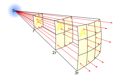
The strength of gravitational force follow the inverse square law distributing gravitational flux over the surface area of a sphere (4πr²).

Inverse Square Law

Any source of a signal strength (S₀) that radiates isotropically in 3-dimensional space will distribute that signal strength (S₀) over the surface area of a sphere (SA = 4πr) of radius (r). Such that the intensity (I) at distance (r) is:

$$I(r) = \frac{S_0}{4 \pi r^{2}}=\frac{S_0}{2 \tau r^{2}}$$ #### Rν Reduced Gravitational Constant In this version of Newton’s Law of Gravity we introduce a new constant G₀, the reduced gravitational constant to accommodate for the factor of 4π = 2τ which is has been integrated in the SI version of the gravitational constant.

$F_g =G \frac{m_{1} m_{2}}{r^{2}}= G_0 \frac{m_{1} m_{2}}{4 \pi r^{2}}=G_0 \frac{m_{1} m_{2}}{2 \tau r^{2}}$

Where:

$G = \frac{G_{0}}{2\tau} = 6.67384 \times 10^{-11} \frac{N \cdot m^2}{kg^2}$

Analyzing the units: $$\frac{N \cdot m^2}{kg^2} = \left( \frac{\left( kg \cdot \frac{m}{s^2} \right) \cdot m^2}{kg^2} \right)=\frac{m^3}{s^2 kg}$$ Converting seconds to meters with the SI speed of light as a conversion factor: $$\frac{m^3}{s^2 kg}\cdot\frac{1}{c^2}=\frac{m^3}{s^2 kg}\cdot\frac{s^2}{m^2}=\frac{m}{kg}$$

Thus where space and time are measured in units of meters, the reduced gravitational constant, is:

$$\boxed{G_0=\frac{2\tau G}{c^2}=\frac{2\tau \cdot 6.67384 \times 10^{-11}}{299792458^2} \frac{m}{kg} = 9.33135 \times 10^-27 \frac{m}{kg}}$$

Observation This implies that not only can space an time be measure in units of meters, but so can mass.

Relativistic Energy Momentum Relation

Einsteins Relativistic Energy Momentum relationship shows a Pythagorean relation between the total energy (E), rest mass (m₀) and momentum (p) of a system.

E² = (m₀⋅c²)² + (p⋅c)²

Where space and time are both measure in units of meters, c=1.

E² = (m₀)² + (p)²

From this we can see that Energy, Momentum and Mass have equivalent units.

While we do not really know what energy, mass and momentum are we know that they are fundamentally “made” out of the same stuff because they have the same units.

Objects of mass at rest

For an object at rest with no momentum (p = 0) we see Einstein’s famous equations:

E = m₀ ⋅ c²

Or, with c = 1, this is much simpler to understand. Energy = Mass

E = m₀

Zero mass objects moving at the speed of light

And for objects with no mass, like photos, (m₀ = 0):

E = pc

Or, with c = 1, this is much simpler to understand. Energy = Momentum

E = p

Planck’s Constant

The Reduced Planck constant , ħ, represents a conversion factor for relating the frequency, ω (in 2π radians per second), of a photon to the energy of that photon. This can easily be seen from the simple but profound relationship:

E = ℏω

Where:

ℏ = 1.054571726 × 10⁻³⁴J ⋅ s

and

$J \cdot s = {kg}\cdot\frac{m^2}{s}$

Reduced Planck’s Constant $\hbar = \frac{h}{2\pi} = \frac{h}{\tau}$

Simplifying our units by converting time and mass to units of meters: $$\boxed{\hbar=1.054571726 \times 10^{−34} {kg}\cdot\frac{m^2}{s}\cdot\frac{G_0}{c}=3.282462\times10^{-69}m^2}$$

Which suggest that the Plank constant can be interpreted as an areas for which the square root of is suspiciously close to the Plank length:

$$\boxed{\sqrt{\hbar}=\sqrt{3.282462\times10^{-69}m^2}=5.72928\times10^{-35}m}$$

Planck Area

The Planck Area is the square of the Planck Length.

$l_{P}= \sqrt{\frac{\hbar G}{c^3}}$

and $l_{P}^{2}= \frac{\hbar G}{c^3}$

In Rν units both c and G_o are 1.

$l_{P} = \sqrt{\hbar}$

and l_P² = ℏ ## Bekenstein’s Bound After having recently read Three Roads to Quantum Gravity by Lee Smolin, I now suspect the meaning of this areas is related to the Bekensteins Law as applied to a surface areas surrounding a mass. Where the thermodynamic entropy, S, is proportional to the the enclosed surface area, A.

$S=\frac{1}{4}\cdot\frac{A}{G\hbar}$

$S=\frac{k c^{3} A}{4 G \hbar}$

$S \le \frac{2\pi k R E}{\hbar c} = \frac{\tau R k E}{\hbar c}$

From our new values for G₀and ℏ we can likely rewrite this:

$S=\frac{\pi\cdot A}{\hbar G_0}$

With the limiting case being at the Plank scale.

$S=\frac{\pi\cdot \sqrt{\hbar}}{\hbar G_0}$

Planck Length

https://en.wikipedia.org/wiki/Planck_length

The concept of the Planck Length comes from exploring the limits of Quantum Mechanics and General Relativity. The limits of General Relativity can be seen a the event horizon of a black hole, described by the Schwarzschild Radius. And the limits of Quantum Mechanics can be found in the Compton Wavelength for a given quanta.

The Schwarzschild Radius is defined as the distance at which light cannot escape from the gravitational field of a mass (m):

Classic Derivation.

$r_S=\frac{2G m}{c^2}$

The reduced Compton Wavelength represents a lower limit on the wavelength for quanta that can interact with a quantum particle with mass (m):

$\lambda_C=\frac{h}{m c}$

$\bar{\lambda_C}=\frac{2\pi\hbar}{m c}=\frac{\tau\hbar}{m c}$

And set the Schwarzschild Radius equal to the Compton Wavelength: r_S = λ_C

$\frac{2Gm}{c^{2}}=\frac{h}{m c}$

$m^{2}= \frac{hc}{2G}$

$m = \sqrt{\frac{hc}{2G}}$

$l_P=\frac{2G\sqrt{\frac{hc}{2G}}}{c^2}$ $l_P=\frac{2G\sqrt{\frac{hc}{2G}}}{c^{2}}= \sqrt{\frac{2Gh}{c^2}}$

With reduced Compton Wavelength $r_S=\bar{\lambda_C}$

$\frac{2Gm}{c^{2}}=\frac{\tau\hbar}{m c}$

$m^2=\frac{\tau\ \hbar\ c}{2G}$

$m = \sqrt{\frac{\tau\ \hbar\ c}{2G}}$

$l_P=\frac{2G\sqrt{\frac{\tau\ \hbar\ c}{2G}}}{c^2}$

$l_P=\frac{2G\sqrt{\frac{\tau\ \hbar\ c}{2G}}}{c^{2}}=\sqrt{\frac{4\ \tau\ G\ \hbar}{c^3}}$

If we reduce the units in these equation to those of mass and time measured in meters.

$l_P=\sqrt{4\tau\hbar G_{o}}$

and

$\lambda_C=\frac{\hbar}{m}$

$m=R_s=\lambda_C=\frac{\hbar}{m}$

This is known as the Planck Mass, M_P. $M_P=m=\sqrt{\hbar}$

Solving the Compton Wavelength for distance we find the classic Plank Length:

$\lambda_C=\frac{\hbar}{\sqrt{\hbar}}=\frac{\sqrt{\hbar}}{\sqrt{\hbar}}\cdot\frac{\hbar}{\sqrt{\hbar}}=\sqrt{\hbar}=L_P$

Which is in precise agreement with the value we found in above. Thus the Plank Length is:

$L_P=\sqrt{\hbar}=5.72928\times10^{-35}m$

When we measure distance, time, and mass in units of distance, c=1, and the Plank Time, T_P, is equal to Plank Length, L_P, which is equal to the Plank Mass, M_P:

$$\boxed{L_P=T_P=M_P}$$

Applying conversion factors from the table above, we can convert SI values to Reduced Natural Units. $c=\frac{1}{\sqrt{\epsilon_o \mu_o}}$

Fine Structure Constant

https://en.wikipedia.org/wiki/Fine-structure_constant As a consistency check, we compute the Fine Structure Constant using Reduced Natural Units which is a unit less ratio that should be independent of our system of units.

$\huge{\alpha=\frac{e^2}{4\pi\epsilon_o\hbar c}=\frac{e^2}{4\pi}=0.00729735≈\frac{1}{137}}$

This check confirms that our system of Reduced Natural Units has internally consistent values for c, ϵ_o, ℏ and e−. And also G_o which was used to computer prior values is also consistent.

Sage Code

Unit Analysis computations have been performed with Sage Math.

# Define constance
one = 1.n(digits=6)
pi = pi.n(digits=6)
tau = 2 * pi
t = tau

# Define the units
meters = var('m')
m = one*meters

seconds = var('s')
s = seconds

kilograms = var('kg')
kg = kilograms

newtons = kg * m / s^2
N = newtons

joules = N * m
J = joules

print("pi    =", pi)
print("tau   =", t)

# Speed of light in meters/second
speed_of_light = 299792458 * meters/seconds
sol = speed_of_light
c = sol
print("si c  =", c)

rnu_c = c / c
print("R\u03BD c  =", rnu_c)

# Gravitational Constant
gravitational_constant = 6.67384e-11 * N*(m^2/kg^2)
G = gravitational_constant
print("si G  =", G)

rnu_G = 4*pi*G/c^2
Go = rnu_G
print("R\u03BD Go =", Go)


# Planck's Constant
reduced_plancks_constant = 1.054571726e-34 * J*s
h_bar = reduced_plancks_constant
print("si \u210F  =", h_bar)

rnu_h_bar = h_bar * Go / c
print("R\u03BD "u"\u210F  =", rnu_h_bar)

# Planck Length
rnu_h_bar_str = str(rnu_h_bar) 
numerical_part_str = rnu_h_bar_str.split('*')[0]  
numerical_part_str = numerical_part_str.strip('()')
numerical_part = float(numerical_part_str)
rnu_sqrt_h_bar = numerical_part^(1/2)
# ^ Sage cannot process sqrt on units... Lame.
lP = rnu_sqrt_h_bar * m
print("R\u03BD \u221A\u210F =", lP)

Output

pi    = 3.14159
tau   = 6.28319
si c  = 299792458*m/s
Rν c  = 1
si G  = (6.67384e-11)*m^3/(kg*s^2)
Rν Go = (9.33135e-27)*m/kg
si ℏ  = (1.05457e-34)*kg*m^2/s
Rν ℏ  = (3.28246e-69)*m^2
Rν √ℏ = (5.72928e-35)*m
si lP = (1.61620e-35)*sqrt(m^2)
Rν lP = (2.77455e-47)*sqrt(m^3/kg)

Terminology

Citations